

Transformer를 공부하다 보면 가장 먼저 마주치는 핵심 개념이 바로 Attention입니다.
2017년 Google이 발표한 《Attention Is All You Need》 논문에서는 RNN이나 CNN 없이 Self-Attention을 중심으로 문장을 처리하는 Transformer 구조를 제안했습니다.
특히 Transformer에서 가장 중요한 흐름은 다음과 같습니다.
Token → Embedding → Positional Encoding → Query / Key / Value → Attention Score → Softmax → Weighted Sum
이번 글에서는 복잡한 라이브러리를 사용하는 대신, 간단한 한국어 문장과 PyTorch 코드를 이용하여 이 과정이 실제로 어떻게 계산되는지 하나씩 살펴보겠습니다.
1. Attention이란?
Attention을 한 문장으로 정의하면 다음과 같습니다.
현재 단어가 다른 단어들을 얼마나 중요하게 참고해야 하는지를 계산하는 방법
예를 들어 다음 문장이 있다고 가정해 보겠습니다.
나는 오늘 학교에 간다
나는이라는 단어를 처리할 때 Transformer는 나는만 보는 것이 아닙니다.
나는 → 나는
나는 → 오늘
나는 → 학교에
나는 → 간다
처럼 문장 안의 다른 모든 단어와 관계를 계산합니다.
마찬가지로 오늘도,
오늘 → 나는
오늘 → 오늘
오늘 → 학교에
오늘 → 간다
를 계산합니다.
즉, 길이가 4인 문장이라면 기본적인 Self-Attention에서는 총
개의 관계가 만들어집니다.
이것이 Self-Attention의 핵심입니다.
2. 전체 코드 흐름
이번 예제에서 구현할 전체 구조는 다음과 같습니다.
문장
 ↓
Token ID
 ↓
Embedding
 ↓
Positional Encoding
 ↓
Query / Key / Value
 ↓
QKᵀ
 ↓
Scale
 ↓
Mask (선택)
 ↓
Softmax
 ↓
Attention Weight
 ↓
Attention Weight × V
 ↓
Attention Output
하나씩 직접 확인해 보겠습니다.
3. Vocabulary 만들기
먼저 단어를 숫자로 변환하기 위한 Vocabulary를 정의합니다.
vocab = {
    "[PAD]": 0,
    "나는": 1,
    "오늘": 2,
    "학교에": 3,
    "간다": 4,
    "도서관에": 5,
    "학교에서": 6,
    "공부한다": 7,
    "집에": 8
}
컴퓨터는 나는, 오늘, 학교에와 같은 문자열 자체를 신경망에 바로 입력할 수 없습니다.
따라서 각각의 단어에 ID를 부여합니다.
[PAD]    → 0
나는     → 1
오늘     → 2
학교에   → 3
간다     → 4
...
4. 여러 문장을 하나의 Tensor로 만들기
다음과 같이 4개의 문장을 사용해 보겠습니다.
x = torch.LongTensor([
    [1, 2, 3, 4],
    [1, 2, 5, 4],
    [2, 1, 6, 7],
    [1, 8, 4, 0]
])
각 행은 하나의 문장을 의미합니다.
[1, 2, 3, 4]
→ 나는 오늘 학교에 간다

[1, 2, 5, 4]
→ 나는 오늘 도서관에 간다

[2, 1, 6, 7]
→ 오늘 나는 학교에서 공부한다

[1, 8, 4, 0]
→ 나는 집에 간다 [PAD]
따라서 x의 Shape은
print(x.shape)
torch.Size([4, 4])
입니다.
즉,
입니다.
5. Embedding
Token ID 자체에는 단어의 의미가 없습니다.
예를 들어
나는 = 1
오늘 = 2
학교에 = 3
이라고 해서 학교에가 나는보다 3배 큰 의미를 가지는 것은 아닙니다.
따라서 각각의 Token을 Vector로 변환해야 합니다.
이를 담당하는 것이 Embedding입니다.
class Embeddings(nn.Module):

    def __init__(self, d_model, vocab_size):

        super().__init__()

        self.lut = nn.Embedding(
            vocab_size,
            d_model
        )

        self.d_model = d_model

    def forward(self, x):

        return self.lut(x) * math.sqrt(self.d_model)
여기서
nn.Embedding(vocab_size, d_model)
은 쉽게 말하면 Embedding Lookup Table입니다.
예를 들어 d_model = 6이라면 각각의 단어는 6차원 Vector를 가지게 됩니다.
나는 → [x₁, x₂, x₃, x₄, x₅, x₆]

오늘 → [y₁, y₂, y₃, y₄, y₅, y₆]
6. 왜 √d_model을 곱할까?
원래 Transformer 구현에서는 Embedding 결과에 다음 값을 곱합니다.
코드에서는
return self.lut(x) * math.sqrt(self.d_model)
입니다.
d_model = 6이라면
이므로 Embedding Vector 전체에 약 2.449가 곱해집니다.
이는 Embedding의 값 크기를 적절하게 조정하여 이후 더해지는 Positional Encoding과의 상대적인 Scale을 맞추기 위한 것입니다.
7. Embedding Shape 확인
d_model = 6

embedding_layer = Embeddings(
    d_model,
    len(vocab)
)

embedding = embedding_layer(x)
입력 Shape은
[4, 4]
이지만 각 Token이 6차원 Vector로 변환되므로 결과는
[4, 4, 6]
이 됩니다.
즉,
입니다.
현재 예제에서는
4개의 문장
×
문장당 4개의 단어
×
단어당 6개의 숫자
입니다.
8. Embedding만으로는 부족한 이유
여기서 중요한 문제가 하나 있습니다.
Embedding은 단어가 문장 어디에 위치하는지 알지 못합니다.
예를 들어
나는 오늘 학교에 간다
와
오늘 나는 학교에 간다
에서 나는의 Embedding Vector는 동일합니다.
하지만 자연어에서는 단어의 위치와 순서가 중요합니다.
Transformer에는 RNN처럼 순서대로 단어를 처리하는 구조가 없기 때문에 위치 정보를 별도로 추가해야 합니다.
이것이 바로 Positional Encoding입니다.
9. Positional Encoding
Transformer 논문에서는 Sin과 Cos 함수를 이용하여 위치 정보를 생성합니다.
공식은 다음과 같습니다.
짝수 차원:
홀수 차원:
코드로 구현하면 다음과 같습니다.
class PositionalEncoding(nn.Module):

    def __init__(self, d_model, max_len=4):

        super().__init__()

        pe = torch.zeros(max_len, d_model)

        position = torch.arange(
            0, max_len
        ).unsqueeze(1).float()

        # a^b = e^(b × ln(a)), a ** b = math.exp(b * math.log(a))
        div_term = torch.exp(
            torch.arange(0, d_model, 2).float()
            *
            (-math.log(10000.0) / d_model)
        )

        pe[:, 0::2] = torch.sin(
            position * div_term
        )

        pe[:, 1::2] = torch.cos(
            position * div_term
        )

        pe = pe.unsqueeze(0)

        self.register_buffer(
            "pe",
            pe
        )

    def forward(self, x):

        return x + self.pe[:, :x.size(1)]
10. 왜 sin과 cos를 사용할까?
핵심은 각 위치마다 서로 다른 Pattern을 만들어 주기 위해서입니다.
예를 들어
Position 0
Position 1
Position 2
Position 3
은 서로 다른 Positional Encoding Vector를 가지게 됩니다.
그리고 각 차원마다 서로 다른 주기의 Sin/Cos 값을 사용합니다.
따라서 Transformer는 단순히
“이 단어가 무엇인가?”
뿐만 아니라
“이 단어가 문장의 몇 번째 위치에 있는가?”
라는 정보도 함께 사용할 수 있습니다.
11. Embedding + Positional Encoding
Positional Encoding은 Embedding과 연결(concatenate)하는 것이 아니라 더합니다.
코드에서는
output = pe(embedding)
입니다.
예를 들어 어떤 단어의 Embedding이
이고 위치 정보가
이라면,
이 됩니다.
즉, 하나의 Vector 안에
단어 정보 + 위치 정보
가 함께 들어갑니다.
12. 이제 Attention으로 들어가 보자
Embedding과 Positional Encoding까지 끝났다면 이제 Transformer의 핵심인 Attention을 계산할 수 있습니다.
Attention 함수는 다음과 같습니다.
def attention(query, key, value, mask=None, dropout=None):

    d_k = query.size(-1)

    scores = torch.matmul(
        query,
        key.transpose(-2, -1)
    ) / math.sqrt(d_k)

    if mask is not None:
        scores = scores.masked_fill(
            mask == 0,
            -1e9
        )

    p_attn = F.softmax(
        scores,
        dim=-1
    )

    if dropout is not None:
        p_attn = dropout(p_attn)

    return torch.matmul(
        p_attn,
        value
    ), p_attn
이 짧은 코드 안에 Transformer Attention의 핵심 원리가 거의 모두 들어 있습니다.
13. Query, Key, Value란?
Attention을 이해하려면 먼저 Q, K, V를 이해해야 합니다.
Query
내가 지금 무엇을 찾고 있는가?
즉, 다른 단어를 조회하는 주체입니다.
Key
나는 어떤 정보를 가지고 있는 단어인가?
Query가 다른 단어를 검색할 때 비교되는 대상입니다.
Value
실제로 전달할 내용은 무엇인가?
Query와 Key의 관계를 계산한 뒤 실제로 가져오는 정보입니다.
검색 엔진에 비유하면 이해하기 쉽습니다.
검색창에 입력한 검색어
        ↓
      Query

검색 대상이 되는 문서의 특징
        ↓
       Key

검색 후 실제로 가져올 문서의 내용
        ↓
      Value
간단히 정리하면,
Query = 찾는 쪽
Key   = 찾아지는 쪽
Value = 찾은 뒤 가져올 실제 내용
이라고 생각할 수 있습니다.
14. 그런데 현재 코드에서는 Q = K = V이다
사용자가 작성한 코드에는 다음 부분이 있습니다.
query = key = value = pe_result
즉,
입니다.
여기서 X는
결과입니다.
따라서 같은 문장 내부의 단어들이 서로를 바라보게 됩니다.
이것이 바로 Self-Attention입니다.
다만 실제 Transformer에서는 보통 그대로 Q = K = V = X를 Attention 함수에 넣지 않습니다.
각각 서로 다른 학습 가능한 Weight Matrix를 사용합니다.
즉,
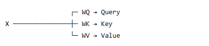
가 실제 Transformer의 구조에 더 가깝습니다.
따라서 현재 코드는 Scaled Dot-Product Attention의 계산 원리를 단순화하여 확인하는 예제라고 보는 것이 정확합니다.
15. Attention의 핵심 공식
Transformer의 Scaled Dot-Product Attention 공식은 다음과 같습니다.
처음 보면 복잡해 보이지만 실제로는 4단계입니다.
① Q와 K 비교
② √dₖ로 나누기
③ Softmax
④ V를 가중합
하나씩 살펴보겠습니다.
16. Step 1 — Query와 Key 비교
코드에서
torch.matmul(
    query,
    key.transpose(-2, -1)
)
부분입니다.
수식으로는
입니다.
예를 들어 입력 Shape이
Q = [batch, sequence, d_k]
K = [batch, sequence, d_k]
라면 K를 transpose하여
Kᵀ = [batch, d_k, sequence]
로 만듭니다.
따라서
결과는
이 됩니다.
17. 왜 [sequence, sequence]가 나올까?
문장이
나는 오늘 학교에 간다
라면 Attention Score Matrix는 개념적으로 다음과 같습니다.
| Query ↓ / Key → | 나는 | 오늘 | 학교에 | 간다 |
|---|---|---|---|---|
| 나는 | score | score | score | score |
| 오늘 | score | score | score | score |
| 학교에 | score | score | score | score |
| 간다 | score | score | score | score |
각 행은 하나의 Query입니다.
예를 들어 첫 번째 행은
"나는"이 "나는"을 얼마나 참고하는가?
"나는"이 "오늘"을 얼마나 참고하는가?
"나는"이 "학교에"를 얼마나 참고하는가?
"나는"이 "간다"를 얼마나 참고하는가?
를 의미합니다.
그래서 문장 길이가 4이면
Attention Score Matrix가 만들어지는 것입니다.
18. Step 2 — 왜 √d_k로 나눌까?
코드에서는 다음 부분입니다.
scores = torch.matmul(
    query,
    key.transpose(-2, -1)
) / math.sqrt(d_k)
즉,
입니다.
Query와 Key의 차원이 커질수록 Dot Product 결과도 커질 가능성이 높습니다.
값이 지나치게 커지면 Softmax가 매우 극단적인 값으로 변할 수 있습니다.
예를 들어
[1, 2, 3]
정도라면 Softmax가 비교적 부드럽게 나오지만,
[10, 20, 30]
처럼 차이가 커지면 가장 큰 값에 확률이 지나치게 집중될 수 있습니다.
그러면 Gradient가 작아져 학습이 불안정해질 수 있습니다.
따라서
로 나누어 Dot Product의 Scale을 조정합니다.
그래서 이름도 Scaled Dot-Product Attention입니다.
쉽게 접근하면 임베딩 차원이 크면 전체적으로 다 커지니 임베딩 차원의 영향을 줄이겠다고는 뜻으로 이해하셔도 됩니다.
19. Step 3 — Mask
다음 코드는 Mask가 존재할 경우 사용됩니다.
if mask is not None:

    scores = scores.masked_fill(
        mask == 0,
        -1e9
    )
Mask의 목적은 특정 위치를 Attention 계산에서 사실상 제거하는 것입니다.
예를 들어
나는 집에 간다 [PAD]
에서 [PAD]는 실제 단어가 아닙니다.
따라서 다른 단어가 [PAD]를 참고하지 못하게 만들 수 있습니다.
Mask된 위치에
-1e9
처럼 매우 작은 값을 넣습니다.
이후 Softmax를 적용하면
이므로 해당 위치의 Attention Probability는 사실상 0이 됩니다.
Decoder에서는 미래 Token을 보지 못하게 하는 Causal Mask도 사용됩니다.
20. Step 4 — Softmax
다음 단계입니다.
p_attn = F.softmax(
    scores,
    dim=-1
)
Softmax를 적용하면 Attention Score가 확률처럼 해석할 수 있는 값으로 변합니다.
예를 들어 나는의 Score가
[1.2, 0.8, 2.4, 0.5]
였다고 가정해 보겠습니다.
Softmax 이후에는 예를 들어
[0.18, 0.12, 0.61, 0.09]
처럼 바뀔 수 있습니다.
합은
입니다.
즉,
나는 → 나는      18%
나는 → 오늘      12%
나는 → 학교에    61%
나는 → 간다       9%
처럼 해석할 수 있습니다.
이 값이 바로 Attention Weight입니다.
코드에서는 p_attn입니다.
21. Step 5 — Attention Weight × Value
마지막 단계입니다.
torch.matmul(
    p_attn,
    value
)
수식으로는
입니다.
예를 들어 Attention Weight가
이라면 최종 결과는
가 됩니다.
즉, 모든 Value를 똑같이 가져오는 것이 아닙니다.
중요한 단어의 Value는 많이 가져오고, 중요하지 않은 단어의 Value는 조금 가져옵니다.
이것이 Attention의 핵심입니다.
22. Attention을 한 문장으로 다시 이해하기
예를 들어 Query가 나는이라고 가정해 보겠습니다.
먼저 나는의 Query와 모든 단어의 Key를 비교합니다.
Q(나는) × K(나는)
Q(나는) × K(오늘)
Q(나는) × K(학교에)
Q(나는) × K(간다)
그 결과를 Softmax하면
나는       0.10
오늘       0.15
학교에     0.25
간다       0.50
가 나왔다고 가정해 보겠습니다.
그러면 최종 나는의 새로운 표현은
가 됩니다.
따라서 Attention 이후의 나는 Vector는 더 이상 단순한 나는의 Embedding이 아닙니다.
문장 전체의 문맥을 반영한 나는의 새로운 표현이 됩니다.
이 부분이 굉장히 중요합니다.
23. Self-Attention의 진짜 의미
처음 Embedding 단계에서
나는
이라는 Vector는 기본적으로 나는이라는 Token 자체의 정보를 가지고 있습니다.
하지만 Self-Attention 이후에는
나는 + 오늘 + 학교에 + 간다
의 관계가 반영됩니다.
즉,
Embedding
→ 단어 자체의 표현

Self-Attention Output
→ 주변 단어와의 관계가 반영된 문맥적 표현
으로 변화합니다.
이 때문에 같은 단어라도 문장에 따라 다른 표현을 가질 수 있습니다.
24. p_attn과 attn의 차이
코드에서는 두 개의 결과를 반환합니다.
return torch.matmul(p_attn, value), p_attn
따라서
attn, p_attn = attention(
    query,
    key,
    value
)
이라고 하면 두 값의 의미가 다릅니다.
p_attn
Attention Weight입니다.
즉,
각 단어가 다른 단어를 얼마나 중요하게 보는가
를 나타냅니다.
Shape은
[batch, sequence, sequence]
입니다.
attn
Attention Weight와 Value를 곱한 최종 결과입니다.
즉,
다른 단어의 정보를 중요도에 따라 가져와 새롭게 만들어진 Vector
입니다.
Shape은
[batch, sequence, d_model]
이 됩니다.
25. Shape으로 전체 흐름 이해하기
예를 들어
batch = 2
sequence = 4
d_model = 512
라고 가정하겠습니다.
Embedding 이후:
[2, 4]
        ↓
Embedding
        ↓
[2, 4, 512]
Positional Encoding 이후에도 Shape은 변하지 않습니다.
[2, 4, 512]
Q, K, V 역시 현재 단순화된 코드에서는
Q = [2, 4, 512]
K = [2, 4, 512]
V = [2, 4, 512]
입니다.
그리고
를 계산하면
[2, 4, 512]
        ×
[2, 512, 4]

        ↓

[2, 4, 4]
가 됩니다.
Softmax 이후에도
p_attn
[2, 4, 4]
입니다.
마지막으로
[2, 4, 4]
      ×
[2, 4, 512]

      ↓

[2, 4, 512]
가 됩니다.
따라서 최종 Attention Output은 다시
[batch, sequence, d_model]
Shape으로 돌아옵니다.
26. 한눈에 보는 Shape 변화
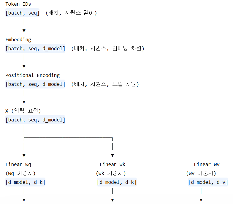
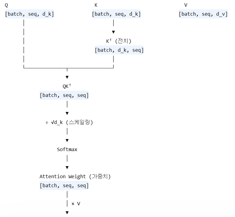

핵심 추가 설명:
- Wq, Wk, Wv는 각각 Query, Key, Value를 만들기 위한 학습 가능한 가중치 행렬입니다.
- 입력 X는 동일하지만 Wq, Wk, Wv가 다르기 때문에 Q, K, V는 서로 다른 표현이 됩니다.
- d_k: Query/Key의 차원 (보통 d_model / head 수)
- d_v: Value의 차원 (보통 d_k와 동일하거나 별도 설정)
- 최종 출력은 각 단어가 “문맥 정보를 반영한 새로운 표현”으로 변환된 결과입니다.
27. 현재 코드에서 반드시 알아야 할 점
현재 코드에서는
query = key = value = pe_result
로 설정했습니다.
Attention의 원리를 공부하기에는 매우 좋은 방법이지만, 실제 Transformer의 Self-Attention 구현과는 한 단계 차이가 있습니다.
실제 Transformer에서는 일반적으로 다음과 같이 학습 가능한 Linear Layer를 사용합니다.
W_Q = nn.Linear(d_model, d_model)
W_K = nn.Linear(d_model, d_model)
W_V = nn.Linear(d_model, d_model)

query = W_Q(pe_result)
key   = W_K(pe_result)
value = W_V(pe_result)
수식으로 표현하면
입니다.
즉, 출발점은 같은 X이지만 서로 다른 Weight를 통과하기 때문에 실제 Q, K, V 값은 서로 달라집니다.
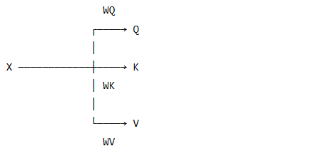
그리고 여기서 한 단계 더 발전하면 각각을 여러 Head로 나누는 Multi-Head Attention으로 이어집니다.
28. 전체 Attention 계산 다시 정리
Transformer Attention의 핵심을 코드 순서 그대로 정리하면 다음과 같습니다.
① 입력 표현 생성
② Query, Key, Value 생성
③ Query와 Key의 유사도 계산
④ Scale 조정
⑤ 필요한 경우 Mask 적용
⑥ Softmax로 Attention Weight 생성
⑦ Value의 Weighted Sum 계산
따라서 최종적으로 우리가 잘 알고 있는 공식이 완성됩니다.
29. Transformer Attention의 핵심은 결국 이것이다
Attention을 처음 보면 Q, K, V, Softmax, Matrix Multiplication 때문에 상당히 복잡해 보입니다.
하지만 본질은 생각보다 단순합니다.
나는 오늘 학교에 간다
라는 문장이 있을 때 Transformer는 각 단어에 대해 질문합니다.
"나는"을 이해하는 데
"오늘"은 얼마나 중요한가?

"학교에"는 얼마나 중요한가?

"간다"는 얼마나 중요한가?
그리고 그 중요도를 숫자로 계산합니다.
Query × Key
      ↓
Attention Score
      ↓
Softmax
      ↓
Attention Weight
그 다음 중요도에 따라 실제 정보를 가져옵니다.
Attention Weight × Value
결과적으로 각각의 단어는 혼자 존재하는 Vector가 아니라 문장 전체의 관계를 반영한 새로운 Vector로 변환됩니다.
이것이 Transformer가 문맥을 이해하는 가장 핵심적인 원리 중 하나입니다.
Attention 전체 코드:
import torch
import torch.nn as nn
import torch.nn.functional as F
import math

# =========================================================
# 0. Seed
# =========================================================

torch.manual_seed(0)


# =========================================================
# 1. Vocabulary
# =========================================================

vocab = {
    "[PAD]": 0,
    "나는": 1,
    "오늘": 2,
    "학교에": 3,
    "간다": 4,
    "도서관에": 5,
    "학교에서": 6,
    "공부한다": 7,
    "집에": 8
}

id_to_token = {
    idx: token
    for token, idx in vocab.items()
}


# =========================================================
# 2. Input
# =========================================================

x = torch.LongTensor([
    [1, 2, 3, 4],   # 나는 오늘 학교에 간다
    [1, 2, 5, 4],   # 나는 오늘 도서관에 간다
    [2, 1, 6, 7],   # 오늘 나는 학교에서 공부한다
    [1, 8, 4, 0]    # 나는 집에 간다 [PAD]
])

print("=" * 70)
print("1. INPUT")
print("=" * 70)

print("x:")
print(x)

print("\nx shape:")
print(x.shape)

print("\nSentences:")

for sentence in x:
    tokens = [
        id_to_token[token.item()]
        for token in sentence
    ]

    print(tokens)


# =========================================================
# 3. Embedding
# =========================================================

class Embeddings(nn.Module):

    def __init__(self, d_model, vocab_size):

        super().__init__()

        self.lut = nn.Embedding(
            vocab_size,
            d_model,
            padding_idx=0
        )

        self.d_model = d_model


    def forward(self, x):

        return self.lut(x) * math.sqrt(self.d_model)


d_model = 6

embedding_layer = Embeddings(
    d_model=d_model,
    vocab_size=len(vocab)
)

embedding = embedding_layer(x)

print("\n" + "=" * 70)
print("2. EMBEDDING")
print("=" * 70)

print("embedding:")
print(embedding)

print("\nembedding shape:")
print(embedding.shape)


# =========================================================
# 4. Positional Encoding
# =========================================================

class PositionalEncoding(nn.Module):

    def __init__(self, d_model, dropout=0.0, max_len=100):

        super().__init__()

        self.dropout = nn.Dropout(
            p=dropout
        )

        pe = torch.zeros(
            max_len,
            d_model
        )

        position = torch.arange(
            0,
            max_len
        ).unsqueeze(1).float()

        div_term = torch.exp(
            torch.arange(
                0,
                d_model,
                2
            ).float()
            *
            (
                -math.log(10000.0)
                /
                d_model
            )
        )

        pe[:, 0::2] = torch.sin(
            position * div_term
        )

        pe[:, 1::2] = torch.cos(
            position * div_term
        )

        pe = pe.unsqueeze(0)

        self.register_buffer(
            "pe",
            pe
        )


    def forward(self, x):

        x = x + self.pe[:, :x.size(1)]

        return self.dropout(x)


positional_encoding = PositionalEncoding(
    d_model=d_model,
    dropout=0.0,
    max_len=100
)

pe_result = positional_encoding(
    embedding
)

print("\n" + "=" * 70)
print("3. POSITIONAL ENCODING")
print("=" * 70)

print("Positional Encoding:")
print(
    positional_encoding.pe[
        :,
        :x.size(1)
    ]
)

print(
    "\nPositional Encoding shape:"
)

print(
    positional_encoding.pe[
        :,
        :x.size(1)
    ].shape
)

print("\nEmbedding + Positional Encoding:")

print(pe_result)

print("\npe_result shape:")
print(pe_result.shape)


# =========================================================
# 5. Q, K, V Linear Layer
# =========================================================

d_k = 6
d_v = 6

W_Q = nn.Linear(
    d_model,
    d_k,
    bias=False
)

W_K = nn.Linear(
    d_model,
    d_k,
    bias=False
)

W_V = nn.Linear(
    d_model,
    d_v,
    bias=False
)

query = W_Q(
    pe_result
)

key = W_K(
    pe_result
)

value = W_V(
    pe_result
)

print("\n" + "=" * 70)
print("4. QUERY / KEY / VALUE")
print("=" * 70)

print("Query:")
print(query)

print("\nQuery shape:")
print(query.shape)

print("\nKey:")
print(key)

print("\nKey shape:")
print(key.shape)

print("\nValue:")
print(value)

print("\nValue shape:")
print(value.shape)


# =========================================================
# 6. Padding Mask
# =========================================================

# x != 0
#
# 실제 Token = True
# PAD        = False

padding_mask = (
    x != vocab["[PAD]"]
)

print("\n" + "=" * 70)
print("5. PADDING MASK")
print("=" * 70)

print("padding_mask:")
print(padding_mask)

print("\npadding_mask shape:")
print(padding_mask.shape)


# Attention score shape:
#
# [batch, query_len, key_len]
#
# padding_mask:
#
# [batch, seq]
#
# 이를
#
# [batch, 1, seq]
#
# 로 변경하면 broadcasting을 통해
# 모든 Query에 동일한 Key padding mask를 적용할 수 있다.

attention_mask = padding_mask.unsqueeze(1)

print("\nattention_mask:")
print(attention_mask)

print("\nattention_mask shape:")
print(attention_mask.shape)


# =========================================================
# 7. Scaled Dot-Product Attention
# =========================================================

def attention(
    query,
    key,
    value,
    mask=None,
    dropout=None
):

    # -----------------------------------------------------
    # Step 1.
    # d_k
    # -----------------------------------------------------

    d_k = query.size(-1)

    print("\n" + "-" * 70)
    print("Attention Step 1: d_k")
    print("-" * 70)

    print("d_k:")
    print(d_k)


    # -----------------------------------------------------
    # Step 2.
    # QK^T
    # -----------------------------------------------------

    raw_scores = torch.matmul(
        query,
        key.transpose(-2, -1)
    )

    print("\n" + "-" * 70)
    print("Attention Step 2: QK^T")
    print("-" * 70)

    print("raw scores:")
    print(raw_scores)

    print("\nraw scores shape:")
    print(raw_scores.shape)


    # -----------------------------------------------------
    # Step 3.
    # Scale
    # -----------------------------------------------------

    scores = (
        raw_scores
        /
        math.sqrt(d_k)
    )

    print("\n" + "-" * 70)
    print("Attention Step 3: QK^T / sqrt(d_k)")
    print("-" * 70)

    print("scaled scores:")
    print(scores)

    print("\nscaled scores shape:")
    print(scores.shape)


    # -----------------------------------------------------
    # Step 4.
    # Mask
    # -----------------------------------------------------

    if mask is not None:

        scores = scores.masked_fill(
            mask == 0,
            -1e9
        )

        print("\n" + "-" * 70)
        print("Attention Step 4: Mask")
        print("-" * 70)

        print("masked scores:")
        print(scores)


    # -----------------------------------------------------
    # Step 5.
    # Softmax
    # -----------------------------------------------------

    p_attn = F.softmax(
        scores,
        dim=-1
    )

    print("\n" + "-" * 70)
    print("Attention Step 5: Softmax")
    print("-" * 70)

    print("attention weights:")
    print(p_attn)

    print("\nattention weights shape:")
    print(p_attn.shape)

    print(
        "\nAttention weight row sums:"
    )

    print(
        p_attn.sum(
            dim=-1
        )
    )


    # -----------------------------------------------------
    # Optional Dropout
    # -----------------------------------------------------

    if dropout is not None:

        p_attn = dropout(
            p_attn
        )


    # -----------------------------------------------------
    # Step 6.
    # Attention Weight × V
    # -----------------------------------------------------

    output = torch.matmul(
        p_attn,
        value
    )

    print("\n" + "-" * 70)
    print("Attention Step 6: Attention Weight × V")
    print("-" * 70)

    print("attention output:")
    print(output)

    print("\nattention output shape:")
    print(output.shape)


    return output, p_attn


# =========================================================
# 8. Attention WITHOUT Mask
# =========================================================

print("\n\n")
print("#" * 70)
print("6. ATTENTION WITHOUT MASK")
print("#" * 70)

attn_no_mask, p_attn_no_mask = attention(
    query=query,
    key=key,
    value=value
)

print("\nFinal Attention Output:")
print(attn_no_mask)

print("\nFinal Attention Output Shape:")
print(attn_no_mask.shape)

print("\nFinal Attention Weight:")
print(p_attn_no_mask)

print("\nFinal Attention Weight Shape:")
print(p_attn_no_mask.shape)


# =========================================================
# 9. Attention WITH Padding Mask
# =========================================================

print("\n\n")
print("#" * 70)
print("7. ATTENTION WITH PADDING MASK")
print("#" * 70)

attn_mask, p_attn_mask = attention(
    query=query,
    key=key,
    value=value,
    mask=attention_mask
)

print("\nFinal Masked Attention Output:")
print(attn_mask)

print(
    "\nFinal Masked Attention Output Shape:"
)

print(attn_mask.shape)

print("\nFinal Masked Attention Weight:")
print(p_attn_mask)

print(
    "\nFinal Masked Attention Weight Shape:"
)

print(p_attn_mask.shape)


# =========================================================
# 10. Check Last Sentence
# =========================================================

print("\n" + "=" * 70)
print("8. LAST SENTENCE ATTENTION WEIGHT")
print("=" * 70)

print(
    "Sentence:"
)

print(
    [
        id_to_token[i.item()]
        for i in x[3]
    ]
)

print(
    "\nWithout Mask:"
)

print(
    p_attn_no_mask[3]
)

print(
    "\nWith Padding Mask:"
)

print(
    p_attn_mask[3]
)


# =========================================================
# 11. Compare PAD Attention
# =========================================================

print("\n" + "=" * 70)
print("9. PAD ATTENTION COMPARISON")
print("=" * 70)

print(
    "Without Mask - attention to PAD:"
)

print(
    p_attn_no_mask[
        3,
        :,
        3
    ]
)

print(
    "\nWith Mask - attention to PAD:"
)

print(
    p_attn_mask[
        3,
        :,
        3
    ]
)


# =========================================================
# 12. Shape Summary
# =========================================================

print("\n" + "=" * 70)
print("10. SHAPE SUMMARY")
print("=" * 70)

print(
    "Input:                 ",
    x.shape
)

print(
    "Embedding:             ",
    embedding.shape
)

print(
    "PE Result:             ",
    pe_result.shape
)

print(
    "Query:                 ",
    query.shape
)

print(
    "Key:                   ",
    key.shape
)

print(
    "Value:                 ",
    value.shape
)

print(
    "Attention Weight:      ",
    p_attn_mask.shape
)

print(
    "Attention Output:      ",
    attn_mask.shape
)
실행 결과:
======================================================================
1. INPUT
======================================================================
x:
tensor([[1, 2, 3, 4],
        [1, 2, 5, 4],
        [2, 1, 6, 7],
        [1, 8, 4, 0]])

x shape:
torch.Size([4, 4])

Sentences:
['나는', '오늘', '학교에', '간다']
['나는', '오늘', '도서관에', '간다']
['오늘', '나는', '학교에서', '공부한다']
['나는', '집에', '간다', '[PAD]']

======================================================================
2. EMBEDDING
======================================================================
embedding:
tensor([[[-0.7741, -5.1812,  0.7894, -3.0945,  0.8573,  0.7548],
         [ 0.2936,  3.0316,  2.7355, -0.6057, -3.3133, -4.1542],
         [ 1.3880,  1.9437,  1.4669, -3.8092, -0.8362,  4.5389],
         [ 1.8376, -1.4342, -0.4247,  0.4494,  3.4032,  3.8857]],

        [[-0.7741, -5.1812,  0.7894, -3.0945,  0.8573,  0.7548],
         [ 0.2936,  3.0316,  2.7355, -0.6057, -3.3133, -4.1542],
         [ 2.3179, -2.0666, -1.5030,  0.0774, -1.2068,  0.6085],
         [ 1.8376, -1.4342, -0.4247,  0.4494,  3.4032,  3.8857]],

        [[ 0.2936,  3.0316,  2.7355, -0.6057, -3.3133, -4.1542],
         [-0.7741, -5.1812,  0.7894, -3.0945,  0.8573,  0.7548],
         [ 1.0770,  0.2754,  1.3308, -0.9679,  0.5034, -1.1031],
         [-1.4037, -1.3603,  1.4558,  3.7770,  4.4574, -1.3510]],

        [[-0.7741, -5.1812,  0.7894, -3.0945,  0.8573,  0.7548],
         [-3.2464,  0.4619, -0.1692, -1.2123, -3.6642, -0.4748],
         [ 1.8376, -1.4342, -0.4247,  0.4494,  3.4032,  3.8857],
         [ 0.0000,  0.0000,  0.0000,  0.0000,  0.0000,  0.0000]]],
       grad_fn=<MulBackward0>)

embedding shape:
torch.Size([4, 4, 6])

======================================================================
3. POSITIONAL ENCODING
======================================================================
Positional Encoding:
tensor([[[ 0.0000,  1.0000,  0.0000,  1.0000,  0.0000,  1.0000],
         [ 0.8415,  0.5403,  0.0464,  0.9989,  0.0022,  1.0000],
         [ 0.9093, -0.4161,  0.0927,  0.9957,  0.0043,  1.0000],
         [ 0.1411, -0.9900,  0.1388,  0.9903,  0.0065,  1.0000]]])

Positional Encoding shape:
torch.Size([1, 4, 6])

Embedding + Positional Encoding:
tensor([[[-0.7741, -4.1812,  0.7894, -2.0945,  0.8573,  1.7548],
         [ 1.1350,  3.5719,  2.7819,  0.3932, -3.3112, -3.1542],
         [ 2.2973,  1.5275,  1.5595, -2.8135, -0.8318,  5.5389],
         [ 1.9787, -2.4242, -0.2859,  1.4397,  3.4097,  4.8857]],

        [[-0.7741, -4.1812,  0.7894, -2.0945,  0.8573,  1.7548],
         [ 1.1350,  3.5719,  2.7819,  0.3932, -3.3112, -3.1542],
         [ 3.2272, -2.4827, -1.4103,  1.0731, -1.2025,  1.6085],
         [ 1.9787, -2.4242, -0.2859,  1.4397,  3.4097,  4.8857]],

        [[ 0.2936,  4.0316,  2.7355,  0.3943, -3.3133, -3.1542],
         [ 0.0674, -4.6409,  0.8358, -2.0956,  0.8594,  1.7548],
         [ 1.9863, -0.1408,  1.4235,  0.0278,  0.5077, -0.1031],
         [-1.2626, -2.3503,  1.5946,  4.7673,  4.4639, -0.3510]],

        [[-0.7741, -4.1812,  0.7894, -2.0945,  0.8573,  1.7548],
         [-2.4049,  1.0022, -0.1228, -0.2134, -3.6621,  0.5252],
         [ 2.7469, -1.8503, -0.3320,  1.4451,  3.4075,  4.8857],
         [ 0.1411, -0.9900,  0.1388,  0.9903,  0.0065,  1.0000]]],
       grad_fn=<AddBackward0>)

pe_result shape:
torch.Size([4, 4, 6])

======================================================================
4. QUERY / KEY / VALUE
======================================================================
Query:
tensor([[[ 1.2239,  2.2964,  1.2813,  1.0936,  0.7165, -1.7191],
         [-2.6246, -1.0561, -0.1049, -1.6372,  0.9921,  2.1937],
         [ 0.0470,  2.7471, -0.5755,  0.2462, -2.2924,  1.5968],
         [ 3.1526,  1.1178,  0.3385,  2.8936, -2.3272, -1.3658]],

        [[ 1.2239,  2.2964,  1.2813,  1.0936,  0.7165, -1.7191],
         [-2.6246, -1.0561, -0.1049, -1.6372,  0.9921,  2.1937],
         [-0.3550,  1.8575,  1.6115,  1.0116, -0.8374,  1.1531],
         [ 3.1526,  1.1178,  0.3385,  2.8936, -2.3272, -1.3658]],

        [[-2.4365, -1.2889, -0.5568, -1.8878,  1.2017,  2.0060],
         [ 1.0358,  2.5291,  1.7332,  1.3443,  0.5069, -1.5313],
         [-0.2228,  0.0272,  0.7659,  0.6973, -0.6102,  0.2712],
         [ 4.0767, -2.2516,  0.1249,  2.8440,  0.5259, -3.6386]],

        [[ 1.2239,  2.2964,  1.2813,  1.0936,  0.7165, -1.7191],
         [-0.5970,  1.0825, -1.0015, -1.6724,  1.7058,  0.8162],
         [ 2.8187,  0.9742,  0.3395,  2.8690, -2.7978, -0.9044],
         [ 0.8235,  0.4755,  0.2022,  0.6413,  0.0809, -0.3544]]],
       grad_fn=<UnsafeViewBackward0>)

Query shape:
torch.Size([4, 4, 6])

Key:
tensor([[[ 1.6903, -0.4694, -0.2075,  0.9411, -0.2868,  0.4465],
         [-1.7227,  1.9624,  0.9190, -0.1430, -1.3703, -1.8792],
         [ 0.0860,  1.5866,  1.7015, -2.6037, -0.8976,  0.4851],
         [ 0.8632, -2.2217,  0.1371, -2.5672,  0.4539,  3.0432]],

        [[ 1.6903, -0.4694, -0.2075,  0.9411, -0.2868,  0.4465],
         [-1.7227,  1.9624,  0.9190, -0.1430, -1.3703, -1.8792],
         [ 0.4778, -2.3336,  0.3024, -1.0988, -0.5632,  0.2381],
         [ 0.8632, -2.2217,  0.1371, -2.5672,  0.4539,  3.0432]],

        [[-1.6073,  2.3287,  0.9064,  0.0801, -1.2454, -1.9093],
         [ 1.5749, -0.8356, -0.1949,  0.7180, -0.4117,  0.4766],
         [-0.7065, -0.2104,  0.2124, -0.9328, -0.4112,  0.3219],
         [ 0.5533, -2.2121, -0.8877, -0.5679,  0.6998,  3.0729]],

        [[ 1.6903, -0.4694, -0.2075,  0.9411, -0.2868,  0.4465],
         [ 1.1529,  1.3896,  0.7598,  1.1016, -0.7588, -1.4081],
         [ 0.4481, -2.2145,  0.2316, -3.0029,  0.4488,  3.0284],
         [ 0.5671, -0.6861,  0.1509, -0.3624, -0.1964,  0.5668]]],
       grad_fn=<UnsafeViewBackward0>)

Key shape:
torch.Size([4, 4, 6])

Value:
tensor([[[ 0.1730,  2.2071,  1.9811,  0.7996, -0.7162, -2.0956],
         [-1.6740, -2.9781,  0.2349, -1.3384, -1.3578,  0.7540],
         [ 0.5720,  0.7385,  0.3565,  0.1997, -1.9077, -1.1988],
         [ 1.5996,  0.7815, -0.2446, -0.5561, -0.2638, -0.2028]],

        [[ 0.1730,  2.2071,  1.9811,  0.7996, -0.7162, -2.0956],
         [-1.6740, -2.9781,  0.2349, -1.3384, -1.3578,  0.7540],
         [ 1.2952,  0.7506,  0.8254,  0.1689, -1.1913,  1.3829],
         [ 1.5996,  0.7815, -0.2446, -0.5561, -0.2638, -0.2028]],

        [[-1.9975, -2.9336, -0.1438, -1.2924, -1.1148,  0.5292],
         [ 0.4965,  2.1627,  2.3598,  0.7536, -0.9592, -1.8708],
         [ 0.3880, -0.9776,  0.8207, -0.7092, -0.7144,  0.1890],
         [-0.6857, -1.7086, -0.7973, -2.2640,  0.8165, -0.3154]],

        [[ 0.1730,  2.2071,  1.9811,  0.7996, -0.7162, -2.0956],
         [-1.8948,  0.7158, -0.6594,  0.4657, -0.7511, -0.6715],
         [ 1.8957,  0.4621, -0.3143, -0.6473, -0.3020,  0.1837],
         [-0.1595,  0.1102, -0.0262, -0.3268, -0.4209, -0.0722]]],
       grad_fn=<UnsafeViewBackward0>)

Value shape:
torch.Size([4, 4, 6])

======================================================================
5. PADDING MASK
======================================================================
padding_mask:
tensor([[ True,  True,  True,  True],
        [ True,  True,  True,  True],
        [ True,  True,  True,  True],
        [ True,  True,  True, False]])

padding_mask shape:
torch.Size([4, 4])

attention_mask:
tensor([[[ True,  True,  True,  True]],

        [[ True,  True,  True,  True]],

        [[ True,  True,  True,  True]],

        [[ True,  True,  True, False]]])

attention_mask shape:
torch.Size([4, 1, 4])


######################################################################
6. ATTENTION WITHOUT MASK
######################################################################

----------------------------------------------------------------------
Attention Step 1: d_k
----------------------------------------------------------------------
d_k:
6

----------------------------------------------------------------------
Attention Step 2: QK^T
----------------------------------------------------------------------
raw scores:
tensor([[[ 7.8123e-01,  5.6679e+00,  1.6042e+00, -1.1583e+01],
         [-4.7648e+00, -2.8952e+00,  2.3567e+00,  1.1395e+01],
         [ 5.1154e-01,  4.8865e+00,  5.5746e+00, -2.9548e+00],
         [ 7.5147e+00,  2.4155e+00, -3.4872e+00, -1.2357e+01]],

        [[ 7.8123e-01,  5.6679e+00, -6.4011e+00, -1.1583e+01],
         [-4.7648e+00, -2.8952e+00,  2.9411e+00,  1.1395e+01],
         [-9.9198e-02,  4.5737e+00, -4.3823e+00, -3.6801e+00],
         [ 7.5147e+00,  2.4155e+00, -3.1936e+00, -1.2357e+01]],

        [[-5.0677e+00, -3.5458e+00,  3.7870e+00,  1.0075e+01],
         [ 8.1959e+00, -7.9325e-01, -2.8513e+00, -1.1674e+01],
         [ 1.4137e+00,  3.5826e-01,  2.1527e-03, -8.5305e-01],
         [-5.1622e+00,  8.3686e+00, -6.4205e+00, -5.3026e+00]],

        [[ 7.8123e-01,  8.6573e+00, -1.2409e+01, -2.1995e+00],
         [-3.0083e+00, -4.2310e+00,  5.3626e+00, -4.9887e-01],
         [ 7.3354e+00,  1.1418e+01, -1.3426e+01, -2.1454e-02],
         [ 1.5489e+00,  2.9078e+00, -3.6000e+00, -2.7789e-01]]],
       grad_fn=<UnsafeViewBackward0>)

raw scores shape:
torch.Size([4, 4, 4])

----------------------------------------------------------------------
Attention Step 3: QK^T / sqrt(d_k)
----------------------------------------------------------------------
scaled scores:
tensor([[[ 3.1893e-01,  2.3139e+00,  6.5492e-01, -4.7289e+00],
         [-1.9452e+00, -1.1820e+00,  9.6212e-01,  4.6522e+00],
         [ 2.0884e-01,  1.9949e+00,  2.2758e+00, -1.2063e+00],
         [ 3.0679e+00,  9.8611e-01, -1.4237e+00, -5.0446e+00]],

        [[ 3.1893e-01,  2.3139e+00, -2.6133e+00, -4.7289e+00],
         [-1.9452e+00, -1.1820e+00,  1.2007e+00,  4.6522e+00],
         [-4.0498e-02,  1.8672e+00, -1.7891e+00, -1.5024e+00],
         [ 3.0679e+00,  9.8611e-01, -1.3038e+00, -5.0446e+00]],

        [[-2.0689e+00, -1.4476e+00,  1.5460e+00,  4.1129e+00],
         [ 3.3460e+00, -3.2384e-01, -1.1641e+00, -4.7661e+00],
         [ 5.7716e-01,  1.4626e-01,  8.7882e-04, -3.4825e-01],
         [-2.1075e+00,  3.4165e+00, -2.6212e+00, -2.1648e+00]],

        [[ 3.1893e-01,  3.5343e+00, -5.0658e+00, -8.9793e-01],
         [-1.2281e+00, -1.7273e+00,  2.1893e+00, -2.0366e-01],
         [ 2.9947e+00,  4.6615e+00, -5.4810e+00, -8.7585e-03],
         [ 6.3232e-01,  1.1871e+00, -1.4697e+00, -1.1345e-01]]],
       grad_fn=<DivBackward0>)

scaled scores shape:
torch.Size([4, 4, 4])

----------------------------------------------------------------------
Attention Step 5: Softmax
----------------------------------------------------------------------
attention weights:
tensor([[[1.0248e-01, 7.5345e-01, 1.4341e-01, 6.5829e-04],
         [1.3251e-03, 2.8428e-03, 2.4261e-02, 9.7157e-01],
         [6.6183e-02, 3.9484e-01, 5.2290e-01, 1.6075e-02],
         [8.8011e-01, 1.0976e-01, 9.8605e-03, 2.6385e-04]],

        [[1.1888e-01, 8.7402e-01, 6.3340e-03, 7.6363e-04],
         [1.3165e-03, 2.8243e-03, 3.0598e-02, 9.6526e-01],
         [1.2280e-01, 8.2736e-01, 2.1370e-02, 2.8465e-02],
         [8.7901e-01, 1.0962e-01, 1.1102e-02, 2.6352e-04]],

        [[1.9089e-03, 3.5531e-03, 7.0912e-02, 9.2363e-01],
         [9.6452e-01, 2.4578e-02, 1.0608e-02, 2.8927e-04],
         [3.8339e-01, 2.4918e-01, 2.1546e-01, 1.5197e-01],
         [3.9500e-03, 9.8996e-01, 2.3633e-03, 3.7301e-03]],

        [[3.8148e-02, 9.5038e-01, 1.7495e-04, 1.1298e-02],
         [2.8667e-02, 1.7402e-02, 8.7407e-01, 7.9856e-02],
         [1.5759e-01, 8.3456e-01, 3.2854e-05, 7.8193e-03],
         [2.9957e-01, 5.2172e-01, 3.6611e-02, 1.4211e-01]]],
       grad_fn=<SoftmaxBackward0>)

attention weights shape:
torch.Size([4, 4, 4])

Attention weight row sums:
tensor([[1.0000, 1.0000, 1.0000, 1.0000],
        [1.0000, 1.0000, 1.0000, 1.0000],
        [1.0000, 1.0000, 1.0000, 1.0000],
        [1.0000, 1.0000, 1.0000, 1.0000]], grad_fn=<SumBackward1>)

----------------------------------------------------------------------
Attention Step 6: Attention Weight × V
----------------------------------------------------------------------
attention output:
tensor([[[-1.1604, -1.9113,  0.4310, -0.8982, -1.3702,  0.1813],
         [ 1.5635,  0.7717, -0.2257, -0.5382, -0.3074, -0.2267],
         [-0.3247, -0.6311,  0.4063, -0.3801, -1.5853, -0.4711],
         [-0.0255,  1.6231,  1.7728,  0.5587, -0.7983, -1.7735]],

        [[-1.4331, -2.3352,  0.4458, -1.0741, -1.2796,  0.4185],
         [ 1.5792,  0.7718, -0.2076, -0.5343, -0.2958, -0.1540],
         [-1.2905, -2.1547,  0.4483, -1.0214, -1.2443,  0.3903],
         [-0.0167,  1.6222,  1.7762,  0.5579, -0.7917, -1.7441]],

        [[-0.6078, -1.6453, -0.6701, -2.1411,  0.6980, -0.2835],
         [-1.9105, -2.7873, -0.0722, -1.2362, -1.1061,  0.4664],
         [-0.6627, -1.0561,  0.5885, -0.8046, -0.6963, -0.2705],
         [ 0.4820,  2.1207,  2.3345,  0.7308, -0.9527, -1.8507]],

        [[-1.7956,  0.7658, -0.5514,  0.4693, -0.7460, -0.7189],
         [ 1.6162,  0.4884, -0.2315, -0.5609, -0.3312,  0.0831],
         [-1.5552,  0.9460, -0.2383,  0.5121, -0.7430, -0.8912],
         [-0.8900,  1.0672,  0.2342,  0.4124, -0.6773, -0.9816]]],
       grad_fn=<UnsafeViewBackward0>)

attention output shape:
torch.Size([4, 4, 6])

Final Attention Output:
tensor([[[-1.1604, -1.9113,  0.4310, -0.8982, -1.3702,  0.1813],
         [ 1.5635,  0.7717, -0.2257, -0.5382, -0.3074, -0.2267],
         [-0.3247, -0.6311,  0.4063, -0.3801, -1.5853, -0.4711],
         [-0.0255,  1.6231,  1.7728,  0.5587, -0.7983, -1.7735]],

        [[-1.4331, -2.3352,  0.4458, -1.0741, -1.2796,  0.4185],
         [ 1.5792,  0.7718, -0.2076, -0.5343, -0.2958, -0.1540],
         [-1.2905, -2.1547,  0.4483, -1.0214, -1.2443,  0.3903],
         [-0.0167,  1.6222,  1.7762,  0.5579, -0.7917, -1.7441]],

        [[-0.6078, -1.6453, -0.6701, -2.1411,  0.6980, -0.2835],
         [-1.9105, -2.7873, -0.0722, -1.2362, -1.1061,  0.4664],
         [-0.6627, -1.0561,  0.5885, -0.8046, -0.6963, -0.2705],
         [ 0.4820,  2.1207,  2.3345,  0.7308, -0.9527, -1.8507]],

        [[-1.7956,  0.7658, -0.5514,  0.4693, -0.7460, -0.7189],
         [ 1.6162,  0.4884, -0.2315, -0.5609, -0.3312,  0.0831],
         [-1.5552,  0.9460, -0.2383,  0.5121, -0.7430, -0.8912],
         [-0.8900,  1.0672,  0.2342,  0.4124, -0.6773, -0.9816]]],
       grad_fn=<UnsafeViewBackward0>)

Final Attention Output Shape:
torch.Size([4, 4, 6])

Final Attention Weight:
tensor([[[1.0248e-01, 7.5345e-01, 1.4341e-01, 6.5829e-04],
         [1.3251e-03, 2.8428e-03, 2.4261e-02, 9.7157e-01],
         [6.6183e-02, 3.9484e-01, 5.2290e-01, 1.6075e-02],
         [8.8011e-01, 1.0976e-01, 9.8605e-03, 2.6385e-04]],

        [[1.1888e-01, 8.7402e-01, 6.3340e-03, 7.6363e-04],
         [1.3165e-03, 2.8243e-03, 3.0598e-02, 9.6526e-01],
         [1.2280e-01, 8.2736e-01, 2.1370e-02, 2.8465e-02],
         [8.7901e-01, 1.0962e-01, 1.1102e-02, 2.6352e-04]],

        [[1.9089e-03, 3.5531e-03, 7.0912e-02, 9.2363e-01],
         [9.6452e-01, 2.4578e-02, 1.0608e-02, 2.8927e-04],
         [3.8339e-01, 2.4918e-01, 2.1546e-01, 1.5197e-01],
         [3.9500e-03, 9.8996e-01, 2.3633e-03, 3.7301e-03]],

        [[3.8148e-02, 9.5038e-01, 1.7495e-04, 1.1298e-02],
         [2.8667e-02, 1.7402e-02, 8.7407e-01, 7.9856e-02],
         [1.5759e-01, 8.3456e-01, 3.2854e-05, 7.8193e-03],
         [2.9957e-01, 5.2172e-01, 3.6611e-02, 1.4211e-01]]],
       grad_fn=<SoftmaxBackward0>)

Final Attention Weight Shape:
torch.Size([4, 4, 4])


######################################################################
7. ATTENTION WITH PADDING MASK
######################################################################

----------------------------------------------------------------------
Attention Step 1: d_k
----------------------------------------------------------------------
d_k:
6

----------------------------------------------------------------------
Attention Step 2: QK^T
----------------------------------------------------------------------
raw scores:
tensor([[[ 7.8123e-01,  5.6679e+00,  1.6042e+00, -1.1583e+01],
         [-4.7648e+00, -2.8952e+00,  2.3567e+00,  1.1395e+01],
         [ 5.1154e-01,  4.8865e+00,  5.5746e+00, -2.9548e+00],
         [ 7.5147e+00,  2.4155e+00, -3.4872e+00, -1.2357e+01]],

        [[ 7.8123e-01,  5.6679e+00, -6.4011e+00, -1.1583e+01],
         [-4.7648e+00, -2.8952e+00,  2.9411e+00,  1.1395e+01],
         [-9.9198e-02,  4.5737e+00, -4.3823e+00, -3.6801e+00],
         [ 7.5147e+00,  2.4155e+00, -3.1936e+00, -1.2357e+01]],

        [[-5.0677e+00, -3.5458e+00,  3.7870e+00,  1.0075e+01],
         [ 8.1959e+00, -7.9325e-01, -2.8513e+00, -1.1674e+01],
         [ 1.4137e+00,  3.5826e-01,  2.1527e-03, -8.5305e-01],
         [-5.1622e+00,  8.3686e+00, -6.4205e+00, -5.3026e+00]],

        [[ 7.8123e-01,  8.6573e+00, -1.2409e+01, -2.1995e+00],
         [-3.0083e+00, -4.2310e+00,  5.3626e+00, -4.9887e-01],
         [ 7.3354e+00,  1.1418e+01, -1.3426e+01, -2.1454e-02],
         [ 1.5489e+00,  2.9078e+00, -3.6000e+00, -2.7789e-01]]],
       grad_fn=<UnsafeViewBackward0>)

raw scores shape:
torch.Size([4, 4, 4])

----------------------------------------------------------------------
Attention Step 3: QK^T / sqrt(d_k)
----------------------------------------------------------------------
scaled scores:
tensor([[[ 3.1893e-01,  2.3139e+00,  6.5492e-01, -4.7289e+00],
         [-1.9452e+00, -1.1820e+00,  9.6212e-01,  4.6522e+00],
         [ 2.0884e-01,  1.9949e+00,  2.2758e+00, -1.2063e+00],
         [ 3.0679e+00,  9.8611e-01, -1.4237e+00, -5.0446e+00]],

        [[ 3.1893e-01,  2.3139e+00, -2.6133e+00, -4.7289e+00],
         [-1.9452e+00, -1.1820e+00,  1.2007e+00,  4.6522e+00],
         [-4.0498e-02,  1.8672e+00, -1.7891e+00, -1.5024e+00],
         [ 3.0679e+00,  9.8611e-01, -1.3038e+00, -5.0446e+00]],

        [[-2.0689e+00, -1.4476e+00,  1.5460e+00,  4.1129e+00],
         [ 3.3460e+00, -3.2384e-01, -1.1641e+00, -4.7661e+00],
         [ 5.7716e-01,  1.4626e-01,  8.7882e-04, -3.4825e-01],
         [-2.1075e+00,  3.4165e+00, -2.6212e+00, -2.1648e+00]],

        [[ 3.1893e-01,  3.5343e+00, -5.0658e+00, -8.9793e-01],
         [-1.2281e+00, -1.7273e+00,  2.1893e+00, -2.0366e-01],
         [ 2.9947e+00,  4.6615e+00, -5.4810e+00, -8.7585e-03],
         [ 6.3232e-01,  1.1871e+00, -1.4697e+00, -1.1345e-01]]],
       grad_fn=<DivBackward0>)

scaled scores shape:
torch.Size([4, 4, 4])

----------------------------------------------------------------------
Attention Step 4: Mask
----------------------------------------------------------------------
masked scores:
tensor([[[ 3.1893e-01,  2.3139e+00,  6.5492e-01, -4.7289e+00],
         [-1.9452e+00, -1.1820e+00,  9.6212e-01,  4.6522e+00],
         [ 2.0884e-01,  1.9949e+00,  2.2758e+00, -1.2063e+00],
         [ 3.0679e+00,  9.8611e-01, -1.4237e+00, -5.0446e+00]],

        [[ 3.1893e-01,  2.3139e+00, -2.6133e+00, -4.7289e+00],
         [-1.9452e+00, -1.1820e+00,  1.2007e+00,  4.6522e+00],
         [-4.0498e-02,  1.8672e+00, -1.7891e+00, -1.5024e+00],
         [ 3.0679e+00,  9.8611e-01, -1.3038e+00, -5.0446e+00]],

        [[-2.0689e+00, -1.4476e+00,  1.5460e+00,  4.1129e+00],
         [ 3.3460e+00, -3.2384e-01, -1.1641e+00, -4.7661e+00],
         [ 5.7716e-01,  1.4626e-01,  8.7882e-04, -3.4825e-01],
         [-2.1075e+00,  3.4165e+00, -2.6212e+00, -2.1648e+00]],

        [[ 3.1893e-01,  3.5343e+00, -5.0658e+00, -1.0000e+09],
         [-1.2281e+00, -1.7273e+00,  2.1893e+00, -1.0000e+09],
         [ 2.9947e+00,  4.6615e+00, -5.4810e+00, -1.0000e+09],
         [ 6.3232e-01,  1.1871e+00, -1.4697e+00, -1.0000e+09]]],
       grad_fn=<MaskedFillBackward0>)

----------------------------------------------------------------------
Attention Step 5: Softmax
----------------------------------------------------------------------
attention weights:
tensor([[[1.0248e-01, 7.5345e-01, 1.4341e-01, 6.5829e-04],
         [1.3251e-03, 2.8428e-03, 2.4261e-02, 9.7157e-01],
         [6.6183e-02, 3.9484e-01, 5.2290e-01, 1.6075e-02],
         [8.8011e-01, 1.0976e-01, 9.8605e-03, 2.6385e-04]],

        [[1.1888e-01, 8.7402e-01, 6.3340e-03, 7.6363e-04],
         [1.3165e-03, 2.8243e-03, 3.0598e-02, 9.6526e-01],
         [1.2280e-01, 8.2736e-01, 2.1370e-02, 2.8465e-02],
         [8.7901e-01, 1.0962e-01, 1.1102e-02, 2.6352e-04]],

        [[1.9089e-03, 3.5531e-03, 7.0912e-02, 9.2363e-01],
         [9.6452e-01, 2.4578e-02, 1.0608e-02, 2.8927e-04],
         [3.8339e-01, 2.4918e-01, 2.1546e-01, 1.5197e-01],
         [3.9500e-03, 9.8996e-01, 2.3633e-03, 3.7301e-03]],

        [[3.8584e-02, 9.6124e-01, 1.7694e-04, 0.0000e+00],
         [3.1155e-02, 1.8913e-02, 9.4993e-01, 0.0000e+00],
         [1.5883e-01, 8.4113e-01, 3.3113e-05, 0.0000e+00],
         [3.4919e-01, 6.0814e-01, 4.2675e-02, 0.0000e+00]]],
       grad_fn=<SoftmaxBackward0>)

attention weights shape:
torch.Size([4, 4, 4])

Attention weight row sums:
tensor([[1.0000, 1.0000, 1.0000, 1.0000],
        [1.0000, 1.0000, 1.0000, 1.0000],
        [1.0000, 1.0000, 1.0000, 1.0000],
        [1.0000, 1.0000, 1.0000, 1.0000]], grad_fn=<SumBackward1>)

----------------------------------------------------------------------
Attention Step 6: Attention Weight × V
----------------------------------------------------------------------
attention output:
tensor([[[-1.1604, -1.9113,  0.4310, -0.8982, -1.3702,  0.1813],
         [ 1.5635,  0.7717, -0.2257, -0.5382, -0.3074, -0.2267],
         [-0.3247, -0.6311,  0.4063, -0.3801, -1.5853, -0.4711],
         [-0.0255,  1.6231,  1.7728,  0.5587, -0.7983, -1.7735]],

        [[-1.4331, -2.3352,  0.4458, -1.0741, -1.2796,  0.4185],
         [ 1.5792,  0.7718, -0.2076, -0.5343, -0.2958, -0.1540],
         [-1.2905, -2.1547,  0.4483, -1.0214, -1.2443,  0.3903],
         [-0.0167,  1.6222,  1.7762,  0.5579, -0.7917, -1.7441]],

        [[-0.6078, -1.6453, -0.6701, -2.1411,  0.6980, -0.2835],
         [-1.9105, -2.7873, -0.0722, -1.2362, -1.1061,  0.4664],
         [-0.6627, -1.0561,  0.5885, -0.8046, -0.6963, -0.2705],
         [ 0.4820,  2.1207,  2.3345,  0.7308, -0.9527, -1.8507]],

        [[-1.8143,  0.7732, -0.5574,  0.4784, -0.7497, -0.7263],
         [ 1.7703,  0.5212, -0.2493, -0.5812, -0.3234,  0.0966],
         [-1.5662,  0.9526, -0.2399,  0.5187, -0.7455, -0.8976],
         [-1.0110,  1.2257,  0.2774,  0.5348, -0.7198, -1.1323]]],
       grad_fn=<UnsafeViewBackward0>)

attention output shape:
torch.Size([4, 4, 6])

Final Masked Attention Output:
tensor([[[-1.1604, -1.9113,  0.4310, -0.8982, -1.3702,  0.1813],
         [ 1.5635,  0.7717, -0.2257, -0.5382, -0.3074, -0.2267],
         [-0.3247, -0.6311,  0.4063, -0.3801, -1.5853, -0.4711],
         [-0.0255,  1.6231,  1.7728,  0.5587, -0.7983, -1.7735]],

        [[-1.4331, -2.3352,  0.4458, -1.0741, -1.2796,  0.4185],
         [ 1.5792,  0.7718, -0.2076, -0.5343, -0.2958, -0.1540],
         [-1.2905, -2.1547,  0.4483, -1.0214, -1.2443,  0.3903],
         [-0.0167,  1.6222,  1.7762,  0.5579, -0.7917, -1.7441]],

        [[-0.6078, -1.6453, -0.6701, -2.1411,  0.6980, -0.2835],
         [-1.9105, -2.7873, -0.0722, -1.2362, -1.1061,  0.4664],
         [-0.6627, -1.0561,  0.5885, -0.8046, -0.6963, -0.2705],
         [ 0.4820,  2.1207,  2.3345,  0.7308, -0.9527, -1.8507]],

        [[-1.8143,  0.7732, -0.5574,  0.4784, -0.7497, -0.7263],
         [ 1.7703,  0.5212, -0.2493, -0.5812, -0.3234,  0.0966],
         [-1.5662,  0.9526, -0.2399,  0.5187, -0.7455, -0.8976],
         [-1.0110,  1.2257,  0.2774,  0.5348, -0.7198, -1.1323]]],
       grad_fn=<UnsafeViewBackward0>)

Final Masked Attention Output Shape:
torch.Size([4, 4, 6])

Final Masked Attention Weight:
tensor([[[1.0248e-01, 7.5345e-01, 1.4341e-01, 6.5829e-04],
         [1.3251e-03, 2.8428e-03, 2.4261e-02, 9.7157e-01],
         [6.6183e-02, 3.9484e-01, 5.2290e-01, 1.6075e-02],
         [8.8011e-01, 1.0976e-01, 9.8605e-03, 2.6385e-04]],

        [[1.1888e-01, 8.7402e-01, 6.3340e-03, 7.6363e-04],
         [1.3165e-03, 2.8243e-03, 3.0598e-02, 9.6526e-01],
         [1.2280e-01, 8.2736e-01, 2.1370e-02, 2.8465e-02],
         [8.7901e-01, 1.0962e-01, 1.1102e-02, 2.6352e-04]],

        [[1.9089e-03, 3.5531e-03, 7.0912e-02, 9.2363e-01],
         [9.6452e-01, 2.4578e-02, 1.0608e-02, 2.8927e-04],
         [3.8339e-01, 2.4918e-01, 2.1546e-01, 1.5197e-01],
         [3.9500e-03, 9.8996e-01, 2.3633e-03, 3.7301e-03]],

        [[3.8584e-02, 9.6124e-01, 1.7694e-04, 0.0000e+00],
         [3.1155e-02, 1.8913e-02, 9.4993e-01, 0.0000e+00],
         [1.5883e-01, 8.4113e-01, 3.3113e-05, 0.0000e+00],
         [3.4919e-01, 6.0814e-01, 4.2675e-02, 0.0000e+00]]],
       grad_fn=<SoftmaxBackward0>)

Final Masked Attention Weight Shape:
torch.Size([4, 4, 4])

======================================================================
8. LAST SENTENCE ATTENTION WEIGHT
======================================================================
Sentence:
['나는', '집에', '간다', '[PAD]']

Without Mask:
tensor([[3.8148e-02, 9.5038e-01, 1.7495e-04, 1.1298e-02],
        [2.8667e-02, 1.7402e-02, 8.7407e-01, 7.9856e-02],
        [1.5759e-01, 8.3456e-01, 3.2854e-05, 7.8193e-03],
        [2.9957e-01, 5.2172e-01, 3.6611e-02, 1.4211e-01]],
       grad_fn=<SelectBackward0>)

With Padding Mask:
tensor([[3.8584e-02, 9.6124e-01, 1.7694e-04, 0.0000e+00],
        [3.1155e-02, 1.8913e-02, 9.4993e-01, 0.0000e+00],
        [1.5883e-01, 8.4113e-01, 3.3113e-05, 0.0000e+00],
        [3.4919e-01, 6.0814e-01, 4.2675e-02, 0.0000e+00]],
       grad_fn=<SelectBackward0>)

======================================================================
9. PAD ATTENTION COMPARISON
======================================================================
Without Mask - attention to PAD:
tensor([0.0113, 0.0799, 0.0078, 0.1421], grad_fn=<SelectBackward0>)

With Mask - attention to PAD:
tensor([0., 0., 0., 0.], grad_fn=<SelectBackward0>)

======================================================================
10. SHAPE SUMMARY
======================================================================
Input:                  torch.Size([4, 4])
Embedding:              torch.Size([4, 4, 6])
PE Result:              torch.Size([4, 4, 6])
Query:                  torch.Size([4, 4, 6])
Key:                    torch.Size([4, 4, 6])
Value:                  torch.Size([4, 4, 6])
Attention Weight:       torch.Size([4, 4, 4])
Attention Output:       torch.Size([4, 4, 6])
30. 최종 요약
이번 코드의 전체 과정을 한 줄로 연결하면 다음과 같습니다.
Token
  ↓
Token ID
  ↓
Embedding
  ↓
× √d_model
  ↓
Positional Encoding
  ↓
X
  ↓
Q / K / V
  ↓
QKᵀ
  ↓
÷ √d_k
  ↓
Mask
  ↓
Softmax
  ↓
Attention Weight
  ↓
× Value
  ↓
Context-aware Representation
그리고 가장 중요한 공식은 단 하나입니다.
이를 자연어로 번역하면 다음과 같습니다.
Query와 Key를 비교하여 각 단어의 중요도를 구하고, 그 중요도만큼 Value의 정보를 가져온다.
그리고 Self-Attention에서는 한 문장 안의 단어들이 서로를 Query와 Key로 바라보면서 관계를 계산합니다.
결국 Transformer의 Attention은 단순히 “어떤 단어가 중요한가?”를 찾는 기술이 아니라,
각 단어를 문장 전체의 문맥을 반영한 표현으로 다시 만드는 과정이라고 이해하는 것이 가장 정확합니다.